Final exam guide for B2: Data Tools, Advanced Lookup, and PivotTables

If you're having trouble with your B2 - Upper-intermediate certification exercises, make sure you can answer "Yes" to these questions before reaching out to a teacher:

• If you are working with Text to Columns: Did you select all the required delimiters (e.g., "Semicolon" and "Space") in the Wizard?

• If you are using Data Validation: Did you type the "Title" and "Input Message" exactly as requested, matching all capitalization and punctuation?

• If you are using lookup functions like VLOOKUP: Did you remember to use 0 or FALSE as the final argument for an exact match?

• If you are working with Pivot Tables: Did you uncheck the "Autofit column widths on update" option before resizing your cells?
  
  

If you’ve answered all these questions and you’re still having issues, check the following guide with common errors in the B2 final exam and how to solve them: 

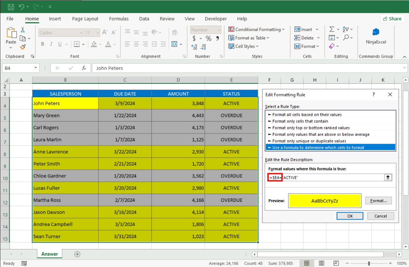
Problem #1: Formula-based Conditional Formatting isn't highlighting the entire row. 
Solution: Check the range in the "Applies to" field within the Rules Manager. It must cover every column in the report (e.g., $B$5:$F$14), not just the column being tested. Also, verify that your formula starts with = and uses the $ sign only before the column letter (e.g., =$E4="ACTIVE").

Problem #2: When using "Text to Columns", the data isn't splitting correctly.

Solution: Review your delimiters in Step 2 of the Wizard. If the task involves specific formats like numbers separated by periods, you must use the "Fixed Width" option and manually place the break lines to include the periods as instructed.

Problem #3: Data Validation is failing or the message isn't appearing.

Solution: The platform requires a 100% exact text match. Check the "Input Message" tab to ensure the Title and Message have no typos or extra spaces. Also, confirm you’ve selected the correct criteria type, such as a "Date" within a specific range.

Problem #4: VLOOKUP + IFERROR isn't displaying the custom error message.

Solution: If the exercise asks for a message like "Locate Salary" to appear during an error, this text must be enclosed in double quotes as the second argument of your IFERROR function. Also, ensure your VLOOKUP uses 0 at the end for an exact match.

Problem #5: The INDEX-MATCH nest is returning a #REF! or #N/A error.

Solution: The "lookup_array" inside your MATCH functions must be a single row or a single column (e.g., B124:B136), never the entire table. One MATCH finds the row index, the other finds the column index. If the formats don't match (e.g., searching for text in a number column), the formula will fail.

Problem #6: The "Show Report Filter Pages" option in the Pivot Table is grayed out.

Solution: This feature only works if the field you want to use for the split (e.g., "Category") is located in the FILTERS area of the PivotTable Field Pane. If that field is currently in "Rows" or "Columns," the option will remain disabled.

Problem #7: Column widths reset every time the Pivot Table is refreshed.

Solution: This is an Excel default that you need to override. Right-click the table > "PivotTable Options" and uncheck the box for "Autofit column widths on update." Do this before you manually adjust your column sizes to ensure they "stick."

Problem #8: Empty cells are appearing instead of zeros in your Pivot Table.

Solution: The platform expects a numeric "0" for missing data, not a blank space. Go to "PivotTable Options," find the field labeled "For empty cells show," and type a 0 in the box. 

Are you still having trouble with a specific B2 task? Check out our related article for more tips on mastering complex data analysis and dynamic reporting!